Week 3 Blog

Date: 14 Feb - 20 Feb

At the supervisor meeting on Monday, we identified the actions to be done by the simulation. There are three motions in total, pitch motion, yaw motion, and roll motion. We have learned the correct way to control the robot to complete the action by consulting the data. Before the research, we thought the simulation of an action is the combination of simple movements of multiple joints. In fact, the correct theory should be to control the motor by calculating the coordinates of each key point on the robot body before and after the movement. The three actions we chose apply the idea of the simulation in three directions of space, respectively. This method requires modeling the robot and applying transformation matrices to calculate the hip and foot positions.

Goals for week 3

1. Research investigates kinematic modeling of quadruped robots.
2. Study the matrix transformation of the coordinate system to calculate the coordinates before and after the action.

Motion computation theory

The modeling calculation of pitch motion

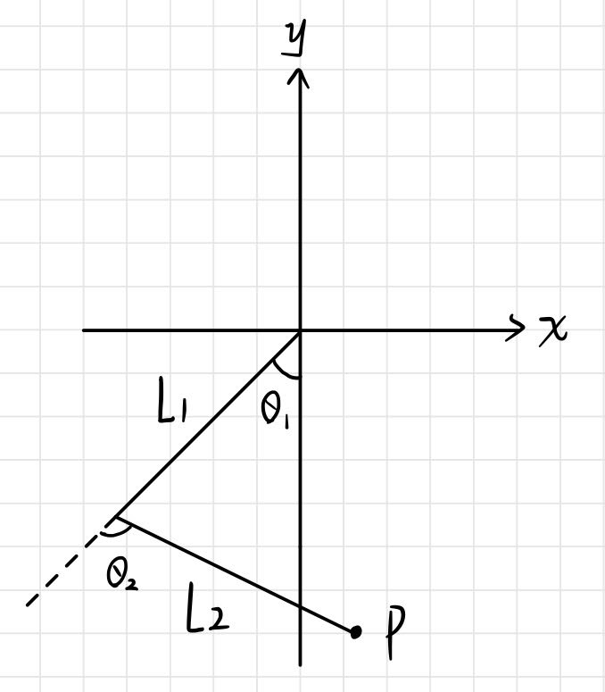
The legs of a quadruped robot can be simplified as a two-bar linkage. In the figure below, is the hip joint angle, is the elbow joint angle, L is the length of the thigh, L is the length of the calf, point P represents the foot, and the x-axis represents the robot body. Among them, L and L are known, and the initial height of the robot is also fixed, so and must be two determined values, which can be obtained by calculation. From this, we can determine the coordinates of point P(x,y).

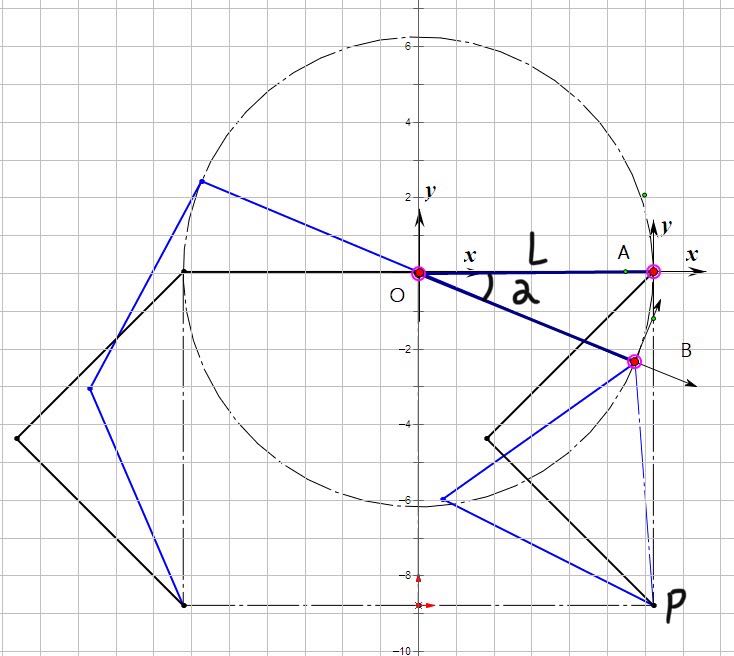
Next, we draw the modeling diagram of the pitch motion. In the picture above, point O is the center point of the robot’s torso, point A is the coordinates of the hip joint before movement, point B is the coordinates after the movement of the hip joint, L is the distance from the hip joint to the midpoint of the body in the current plane and is the angle of leaning over. In the above steps we got the coordinates of point P in the stationary state. Next, we move the coordinate system from point A to point O, then rotate the coordinate system clockwise by angle, and then translate to point B. Find the coordinates of point P in the current coordinate system of point B, and the work is completed. This uses the coordinate system transformation matrix and coordinate transformation matrix knowledge in linear algebra.

AO coordinate system transformation matrix:

OB coordinate system transformation matrix:

The coordinate of point P in the coordinate system of point B is:

Next, the angles and at the two joints can be solved by inverse kinematics. Calculate as follows:

With the changed angles and , we know the angle that the motors at the two joints need to rotate.

In summary, once we have designed the angle, the simulation of the pitch motion can be completed.

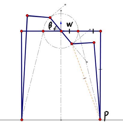
The modeling calculation of roll motion

W is the distance from the hip joint to the midpoint of the fuselage in the current plane. is the angle of rolling. Others are similar to the pitch motion.

The two transformation matrices are:

The coordinates of point P after the movement are:

Then, the two angles at the joint can be solved by inverse kinematics.

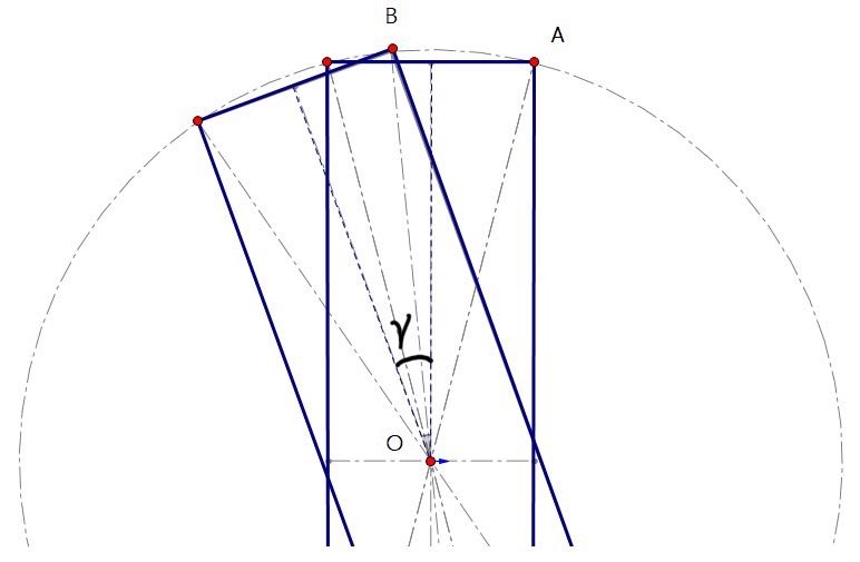
The modeling calculation of yaw motion

is the angle of yawing.

The two transformation matrices are:

The coordinates of point P after the movement are:

Then, the two angles at the joint can be solved by inverse kinematics.

Week 3 summary

This week we successfully modeled three actions. After modeling, the changes of each variable before and after the action were deduced. The feasibility of the project is verified at the theoretical level. Next, we will start writing the code to complete the simulation of the three actions in pybullet.